Task 10 Write a programme for plotting the ideal high-frequency capacitance voltage plot.

This task ask us to write a programme to plot the ideal C-V curve. Our group used matlab to obtain the ideal C-V curve. Firstly, we just get the shift voltage in midgap condition and shift the real C-V curve. however, this method is wrong, the shift voltage is changing in different conditions. Therefore, we know that the ideal curve is not just shift by the real C-V curve. After ten days hard working,  we calculate the gate voltage in different regions refer to the file that tutor given. The result would be shown in the figure 1. The specific code would be shown in the report appendix.

Figure 1

Task 9 Compare your results with results of other group

We got the results of other groups from the tutor. These results could be analyzed to this table  

.seen below table 1. 

From the table, we could see that the higher percentages of Hafnium, the higher permittivity we get. Therefore this material HfSiO called high-k material which the perimittivity is high. However, the value in the last column shows that the value of fixed oxide charge, Nf, the absolute value accumulates while percentage of Hf increases. In conclusion, the alteration of Hf percentage provides a higher permittivity in order to prevent the leakage of current. This is a significant reason that we use the high-k material to replace the dioxide silicon.  

Task-8 Find the oxide charge density at the flatband condition (taking into account the work function difference) and at the midgap condition? How many charges does this correspond to ?

-       Flatband  Condition:                                                                                                                                      From the reading notes, we could write the below equations:

s After calculation 

   

c 

   Midgap Condition:

  The ideal gate voltage could be calculated by the equation

From this equation we know that 

           

The oxide charge density: 

Therefore:

                           

And the correspond charges are 

 After calculation

Task-7 Calculate the midgap voltage

The midgap voltage can be found by figuring out the midgap capacitance first. By definition, the midgap capacitance is a series capacitance with the oxide capacitance (which is the maximum capacitance) and the depletion capacitance, namely,

where

From the lecture note, we obtain an important information, which is that the under midgap condition,

therefore:

The interpretations of the required variables are listed below:

Permittivity in free space - 8.85e(-12) F/M
Relative permittivity for silicon – 11.7
Charge carried by an electron – 1.602*10^(-19) C
Maximum capacitance (read from the given txt file) -2.92*10^3 pF

After calculation

From the txt file, we can figure out the midgap voltage is between 1.36 and 1.37 volts.

 

 

Task-6 Calculate the flatband voltage.

The flatband condition is defined as the applied voltage is 0, and in this case, the capacitance equals to the oxide capacitance in series with the Debye capacitance. Which is:

From the reference handout

Where the Debye capacitance

The interpretation of the required variables are listed below:

Permittivity in free space - 8.85e(-12) F/M

Relative permittivity for silicon – 11.7

Charge carried by an electron – 1.602e(-19)

Maximum capacitance (read from the given txt file) - 2.919e3 pF

Acceptor concentration –  4.088e(21) /m^3

Capacitor area – 2.375829444e(-7)

Thermal voltage – 25 mV

Therefore,

The flatband capacitance is

According to the txt file, the flatband voltage should be in the interval between 0.93 and 0.94 V.

Task-5 Calculate the work function difference assuming a gold (Au) gate.

Work function is defined as the energy difference from the ‘fermi-level’ to the ‘vacuum level’. 

For a metal,  work function is a constant that can be measured. 

For a semiconductor

, where  Xs is electron affinity, and is 4.14eV for silicon.  Eg is the band gap energy and is 1.1eV for silicon, Finally,  the last term is the Fermi level relative to the middle of the band gap, and can be calculated using formula .

Therefore

The function difference is

Task-4 Determine the doping density of the silicon substrate

Doping density I associated with the work function which is links the capacitance. One equation can be used to synthesise the donor’s concentration.

The interpretation for the physical quantities are listed underneath:

Capacitor area – 2.37589444e(-7)/m^2

Charge carried by an electron – 1.602e-(19) C

Boltzmann’s constant – 

Room temperature – 300 K

Permittivity in free space - 8.85e(-12) F/m

Relative permittivity for silicon – 11.2

Silicon intrinsic carrier concentration –  10e15/m^3 

Minimum capacitance (read from the given txt file) – 53.4 pF

Maximum capacitance (read from the given txt file) - 2.919e3 pF

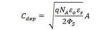
Simplify the equation, we have

The result is a transcendental function of , and MATLAB was utilized to obtain the value of . Two methods were used.

-       Method 1: Adopting the build-in function

The answer is clearly wrong because it indicate there is no doping on the semiconductor.

-       Method 2: Adopting the image method

Separate the equation with the right hand side as

 , and left hand side as

After running the above program, a graph containing two curves was displayed on screen.

The linear line represents for the equation 

and the curve represents for the right hand side equation 

Clearly, the intersection is the desired value for 

Because of the intersection is between 4e21 and 5e21, the domain of the doping concentration could be reduce to an interval between 3.5e21 and 5e21. The result is shown in figure 2.

In order to acquire a more accurate value of doping concentration,  ‘Data cursor’ under the tool bar was utilized and the final approximation value is shown below:

Therefore, the doping concentration is approximately equal to 4.088e21/m^3